Use Tabular Parser
It is very common to export measurement data into a tabular format such as .csv or .xlsx. Following, we'll explore how to utilize NOMAD's tabular parser effectively to enhance our data documentation and visualization.
Our objectives are:
- To upload our
.csvor.xlsxdata files onto NOMAD as entries, so that we can visualize and publish them and make it possible to get a DOI. - Enhance our custom schema by making NOMAD parse the data within these files, and then visualize the data in plots that can be viewed in our customized ELN.
NOMAD offers a versatile tabular parser that can be configured to process tabular data with different representations:
-
Column Mode: each column contains an array of cells that we want to parse into one quantity. Example: current and voltage arrays to be plotted as x and y.
-
Row Mode: each row contains a set of cells that we want to parse into a section, i.e., a set of quantities. Example: an inventory tabular data file (for substrates, precursors, or more) where each column represents a property and each row corresponds to one unit stored in the inventory.
More details on the different representations of tabular data can be found in NOMAD documentation on how to parse tabular data.
Steps to Utilize NOMAD's Tabular Parser for .csv Data
We use an example .csv file, which is the output of an optical absorption instrument. You can find the P3HT_optical.csv file in tutorial_16_materials/part_4_files or download it here. We open this file using Notepad and have a quick look:
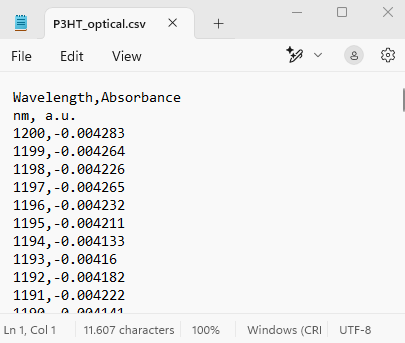
In this .csv file:
- Headers are Wavelength and Absorbance.
- Line 2 gives the units, that we will not need, because we manually define them in the schema.
- Then we have the values for Wavelength and Absorbance, in column mode, as an array.
- The seperator is:
,
Knowing this, we continue to utilize the NOMAD parser with following steps.
Step 1: Defining and Saving the Schema File
Let's start by creating a new schema file with the .archive.yaml format, and create a section called Optical_absorption.
definitions:
  name: This is a parser for optical absorption data in the .csv format
  sections:
    Optical_absorption:
Step 2: Adding the Needed Base Sections
The next step is to inherit the base sections to meet our ELN needs.
- To create entries from this schema we will use
nomad.datamodel.data.EntryData - To use the tabular parser we will use
nomad.parsing.tabular.TableData - To enable the plot function we will use
nomad.datamodel.metainfo.plot.PlotSection
remember, the NOMAD syntax to include sections to inherit from, was base_sections:, and also care for the indentation, base_sections should be indented with respect to the 'Optical_absorption'.
base_sections:
  - nomad.datamodel.data.EntryData
  - nomad.parsing.tabular.TableData
  - nomad.datamodel.metainfo.plot.PlotSection
Step 3: Defining the Quantities of Our Schema
We will define the quantities in our ELN schema. Three quantities are needed, let's call them:
data_fileto upload the data file and apply the tabular parser.wavelengthto store x-axis values extracted by the parser.absorptionto tore y-axis values extracted by the parser.
and give them a proper type and shape attribute.
quantities:
  data_file:
    type: str
  wavelength:
    type: np.float64
    unit: nm
    shape: ['*']
  absorbance:
    type: np.float64
    shape: ['*']
Step 4: Instructing NOMAD on How to Treat Different Quantities
Remember, the syntax for this purpose was m_annotations:
- The
data_filequantity:
The first one is to instruct NOMAD to allow for droping and selecting files in this quantity. Here we will use the following:
The second one is to instruct NOMAD to open the operating system's data browser to select files: The third one instructs NOMAD to apply the tabular parser to extract the data from the uploaded file:tabular_parser:
parsing_options:
comment: '#'
skiprows: [1]
mapping_options:
- mapping_mode: column
file_mode: current_entry
sections:
- '#root'
skiprows can be an integer (e.g., n) or a list of integers. If this is an integer, the parser skips that number of rows and starts from the next one (n+1). If this is a list (e.g., [m, n]), the parser skips the (m+1)th and (n+1)th rows (Python list). Here we have [1], meaning that the 2nd row (the units) will be skipped. We required that, because we needed capture the rest of the column as float numbers.
So we will annotate the data_file as following:
m_annotations:
eln:
  component: FileEditQuantity
browser:
  adaptor: RawFileAdaptor
tabular_parser:
  parsing_options:
    comment: '#'
    skiprows: [1]
  mapping_options:
    - mapping_mode: column
      file_mode: current_entry
      sections:
        - '#root'
-
The
Note that the value for thewavelengthquantity:
This quantitiy will accept values, that will be extracted by the tabular parser. Therefore the annotation will be:namekey must be exactly written as the header of the column that we want to capture its values and put in thewavelengthquantity we defined in the schema. -
The
Again note that the value for theabsorbancequantity:
namekey must be exactly written as the header of the column that we want to capture its values and put in theabsorbancequantity we defined in the schema.
Step 5: Creating a Plot for Your Data
To visualize the data from the uploaded and parsed file within the ELN, we will use an annotation for the main section of our schema Optical_absorption.
By using the plotly_graph_object annotation we instruct NOMAD which quanty should be used for the x-axis and which quanty for the y-axis (can also be several quantities, showing several curves in one plot), as well as provide the title of the plot. Within the plotly_graph_object annotation, the data key defines the quantites for each axis. Here, these varaiable names match those which are defined in the schema. Finally, plot's title is set using the layout key.
m_annotations:
plotly_graph_object:
data:
x: "#wavelength"
y: "#absorbance"
layout:
title: Optical Spectrum
Optical_absorption section definition. Therefore, the m_annotations: must be at the same hierarchy level as quantities, and base_sections.
Step 6 (optional): Adding a Free Text Field
If you only want to publish your data and graph, consider adding a short description.
To do this, select a free text field from editable quantities and add it to your schema.
For example:
Finally our custom schema file should look like the following. You can also find the optical_absorptoion_plot_schema.archive.yaml file in tutorial_16_materials/part_4_files or download it here.
definitions:
name: This is a parser for optical absorption data in the .csv format
sections:
Optical_absorption:
base_sections:
- nomad.datamodel.data.EntryData
- nomad.parsing.tabular.TableData
- nomad.datamodel.metainfo.plot.PlotSection
quantities:
info_about_data:
type: str
m_annotations:
eln:
component: RichTextEditQuantity
data_file:
type: str
m_annotations:
  eln:
    component: FileEditQuantity
  browser:
    adaptor: RawFileAdaptor
  tabular_parser:
    parsing_options:
      comment: '#'
      skiprows: [1]
    mapping_options:
      - mapping_mode: column
        file_mode: current_entry
        sections:
          - '#root'
wavelength:
type: np.float64
unit: nm
shape: ['*']
m_annotations:
  tabular:
    name: Wavelength
absorbance:
type: np.float64
shape: ['*']
m_annotations:
  tabular:
    name: Absorbance
m_annotations:
  plotly_graph_object:
    data:
      x: "#wavelength"
      y: "#absorbance"
    layout:
      title: Optical Spectrum
Step 7: Uploading the Schema File to NOMAD and Creating an Entry
Now that we have created the ELN schema file for parsing the optical absorption data file, let's put it to the test in the NOMAD GUI.
Example: Adding Plot to the Polymer Processing custom schema (Steps)
Now, let's enhance our Polymer Processing schema to include the tabular parser and the plot. We already made the following custom schema polymer_processing_schema.archive.yaml. You simply copy the snippet or download it here.
definitions:
  name: Processing and characterization of polymers thin-films, given by user (gbu)
  sections:
    Experiment_Information_gbu:
      base_sections:
        - nomad.datamodel.data.EntryData
      quantities:
        Name_gbu:
          type: str
          default: Experiment title
          m_annotations:
            eln:
              component: StringEditQuantity
        Researcher_gbu:
          type: str
          default: Name of the researcher who performed the experiment
          m_annotations:
            eln:
              component: StringEditQuantity
        Date_gbu:
          type: Datetime
          m_annotations:
            eln:
              component: DateTimeEditQuantity
        Additional_Notes_gbu:
          type: str
          m_annotations:
            eln:
              component: RichTextEditQuantity
      sub_sections:
        Sample_gbu:
          section:
            base_sections:
              - nomad.datamodel.data.EntryData
              - nomad.datamodel.metainfo.eln.Sample
            m_annotations:
              eln:
                overview: true
                hide: ['chemical_formula']
        Solution_gbu:
          section:
            base_sections:
              - nomad.datamodel.data.EntryData
              - nomad.datamodel.metainfo.eln.Sample
            m_annotations:
              eln:
                overview: true
                hide: ['chemical_formula', 'description']
            quantities:
              Concentration_gbu:
                type: np.float64
                unit: mg/ml
                m_annotations:
                  eln:
                    component: NumberEditQuantity
            sub_sections:
              Solute:
                section:
                  base_sections:
                    - nomad.datamodel.data.EntryData
                  quantities:
                    Substance_gbu:
                      type: nomad.datamodel.metainfo.eln.ELNSubstance
                      m_annotations:
                        eln:
                          component: ReferenceEditQuantity
                    Mass_gbu:
                      type: float
                      unit: kilogram
                      m_annotations:
                        eln:
                          component: NumberEditQuantity
                          defaultDisplayUnit: milligram
              Solvent_gbu:
                section:
                  base_sections:
                    - nomad.datamodel.data.EntryData
                  quantities:
                    substance_gbu:
                      type: nomad.datamodel.metainfo.eln.ELNSubstance
                      m_annotations:
                        eln:
                          component: ReferenceEditQuantity
                    Volume_gbu:
                      type: float
                      unit: meter ** 3
                      m_annotations:
                        eln:
                          component: NumberEditQuantity
                          defaultDisplayUnit: milliliter
        Preparation_gbu:
          section:
            base_sections:
              - nomad.datamodel.data.EntryData
              - nomad.datamodel.metainfo.eln.Process
            m_annotations:
              eln:
                overview: true
We can add the tabular parser and the plot in various places. Here, for the sake of simplicity, we add it as a subsection of the main section, at the same hierarchy level of Sample_gbu, Solution_gbu, and Preparation_gbu. Since it will be itself a section (subsection is a section itself), we should give a section definition using the key section: (see guideline 4 for building custom ELN schemas).
section:. Optionally, we can benefit from a more specialized NOMAD base section nomad.datamodel.metainfo.basesections.Measurement instead of nomad.datamodel.data.EntryData. This gives us more functionalities than just making an entry.
You can also find the polymer_processing_and_optical_absorptoion_plot_schema.archive.yaml file in tutorial_16_materials/part_4_files or download it here.