2D Scatter

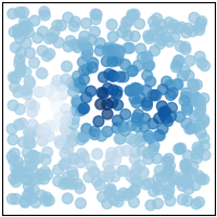
Scatter data in two dimensions.

The x-axis and y-axis define the coordinates of the scattered points.

@NX_class = "NXroot"
@default = "scan1"
scan1:
  @NX_class = "NXentry"
  @default = "data"
  data:
    @NX_class = "NXdata"
    @x_indices = [0]
    @y_indices = [0]
    @signal = "z"
    x: NX_FLOAT64[500]
    y: NX_FLOAT64[500]
    z: NX_FLOAT64[500]

Explanation:

1. @axes is omitted since default axes are not applicable.

2. z is the default signal to be plotted versus x and y.

3. Each data point in z has a coordinate in x and y.

Note that the NXdata structure does not describe how the data needs to be plotted. In this example we create a 2D scatter plot in the XY-plane. But the data could also be plotted as a function of x or y in a Curve plot. When defining @axes="x" the curve plot would be the most likely intention of the data publisher but it is up to the reader to decide how to plot the data.

# Data
import numpy as np

rstate = np.random.RandomState(42)
x = rstate.uniform(-3, 3, 500)
y = rstate.uniform(-3, 3, 500)
z = (1 - x / 2 + x**5 + y**3) * np.exp(-(x**2) - y**2)

# Plot
import matplotlib.pyplot as plt  # noqa E402

plt.style.use("_mpl-gallery-nogrid")

fig, ax = plt.subplots()
ax.scatter(x, y, c=z, s=50, alpha=0.7)

plt.show()