2.3.3.3.171. NXxps
Status:
application definition (contribution), extends NXmpes
Description:
This is the application definition for X-ray photoelectron spectroscopy.
Symbols:
No symbol table
- Groups cited:
NXbeam, NXcalibration, NXcollectioncolumn, NXcoordinate_system, NXdata, NXelectronanalyzer, NXenergydispersion, NXentry, NXfit_function, NXfit, NXinstrument, NXparameters, NXpeak, NXsample, NXsource, NXtransformations
Structure:
definition: (required) NX_CHAR ⤆
Obligatory value:
NXxpsA name of the experimental method according to `Clause 11`_ of ...
A name of the experimental method according to Clause 11 of the ISO 18115-1:2023 specification.
- Examples for XPS-related experiments include:
X-ray photoelectron spectroscopy (XPS)
angle-resolved X-ray photoelectron spectroscopy (ARXPS)
ultraviolet photoelectron spectroscopy (UPS)
hard X-ray photoemission spectroscopy (HAXPES)
near ambient pressure X-ray photoelectron spectroscopy (NAPXPS)
electron spectroscopy for chemical analysis (ESCA)
transitions: (recommended) NX_CHAR ⤆
xps_coordinate_system: (recommended) NXcoordinate_system ⤆
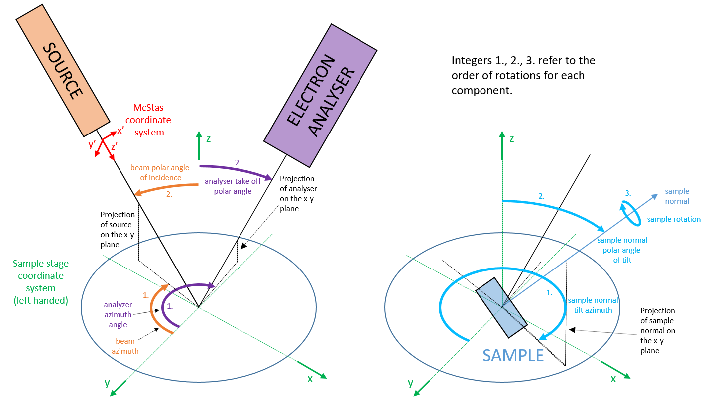
In traditional surface science, a left-handed coordinate system is used such ...
In traditional surface science, a left-handed coordinate system is used such that the positive z-axis points along the normal of the sample stage, and the x- and y-axes lie in the plane of the sample stage. However, in NeXus, a coordinate system that is the same as McStas is used. xps_coordinate_system gives the user the opportunity to work in the traditional base coordinate system.
Obligatory value:
sample stagez_direction: (required) NX_CHAR ⤆
Obligatory value:
sample stage normalObligatory value:
[-1, 0, 0]Obligatory value:
[0, 1, 0]Obligatory value:
[0, 0, 1]depends_on: (required) NX_CHAR ⤆
Link to transformations defining the XPS base coordinate system, ...
Link to transformations defining the XPS base coordinate system, which is defined such that the positive z-axis points along the sample stage normal, and the x- and y-axes lie in the plane of the sample stage.
TRANSFORMATIONS: (optional) NXtransformations ⤆
Set of transformations, describing the orientation of the XPS coordinate s ...
Set of transformations, describing the orientation of the XPS coordinate system with respect to the beam coordinate system (.) or another coordinate system. The transformations in the
NXtransformationsgroup depend on the actual instrument geometry. If the z-axis is pointing in the direction of gravity (i.e., if the sample is mounted horizontally), the following transformations can be used for describing the XPS coordinate system with respect to the beam coordinate system (.):xps_coordinate_system:NXcoordinate_system depends_on=coordinate_transformations/sample_stage_to_source_azimuth coordinate_transformations:NXtransformations sample_stage_to_source_azimuth=beam_azimuth_angle @depends_on=sample_stage_to_source_polar @transformation_type=rotation @vector=[0, 0, -1] @units=degree sample_stage_to_source_polar=beam_polar_angle_of_incidence @depends_on=. @transformation_type=rotation @vector=[1, 0, 0] @units=degreeNote that this
NXtransformationsgroup is not needed when the defined transformations in beam_probe are used. In this case, this group shall not be written here to avoid circular references in the transformations chain.INSTRUMENT: (required) NXinstrument ⤆
Description of the XPS spectrometer and its individual parts. ...
Description of the XPS spectrometer and its individual parts.
This concept is related to term 12.58 of the ISO 18115-1:2023 standard.
source_probe: (recommended) NXsource ⤆
beam_probe: (required) NXbeam ⤆
depends_on: (recommended) NX_CHAR ⤆
Reference to the transformation describing the direction of the beam ...
Reference to the transformation describing the direction of the beam relative to a defined coordinate system.
Should point to /entry/instrument/beam_probe/transformations/beam_direction.
transformations: (recommended) NXtransformations ⤆
beam_direction: (required) NX_NUMBER {units=NX_TRANSFORMATION} ⤆
beam_polar_angle_of_incidence: (required) NX_NUMBER {units=NX_ANGLE} ⤆
Incidence angle of the beam with respect to the upward z-direction, de ...
Incidence angle of the beam with respect to the upward z-direction, defined by the sample stage.
@transformation_type: (required) NX_CHAR ⤆
Obligatory value:
rotation@vector: (required) NX_NUMBER ⤆
Obligatory value:
[-1, 0, 0]@depends_on: (required) NX_CHAR ⤆
Obligatory value:
beam_azimuth_anglebeam_azimuth_angle: (required) NX_NUMBER {units=NX_ANGLE} ⤆
Azimuthal rotation of the beam from the y-direction defined by the sample stage.
@transformation_type: (required) NX_CHAR ⤆
Obligatory value:
rotation@vector: (required) NX_NUMBER ⤆
Obligatory value:
[0, 0, 1]@depends_on: (required) NX_CHAR ⤆
This should point to the coordinate system defined in /entry/xps_coordinate_system.
ELECTRONANALYZER: (required) NXelectronanalyzer ⤆
work_function: (required) NX_FLOAT ⤆
depends_on: (recommended) NX_CHAR ⤆
Reference to the transformation describing the orientation of the analyz ...
Reference to the transformation describing the orientation of the analyzer relative to a defined coordinate system.
transmission_function: (recommended) NXdata ⤆
COLLECTIONCOLUMN: (required) NXcollectioncolumn ⤆
magnification: (recommended) NX_FLOAT {units=NX_DIMENSIONLESS} ⤆
ENERGYDISPERSION: (required) NXenergydispersion ⤆
transformations: (recommended) NXtransformations ⤆
analyzer_take_off_polar_angle: (required) NX_NUMBER {units=NX_ANGLE} ⤆
Polar tilt of the analyzer with respect to the upward z-direction, def ...
Polar tilt of the analyzer with respect to the upward z-direction, defined by the sample stage.
The angle between the incoming beam and the analyzer is given by beam_analyzer_angle = beam_polar_angle_of_incidence + analyzer_take_off_polar_angle. In practice, the analyzer axis is often set as the z axis (analyzer_take_off_polar_angle = 0), so that beam_analyzer_angle = beam_polar_angle_of_incidence. For magic angle configurations, this angle is 54.5°.
@transformation_type: (required) NX_CHAR ⤆
Obligatory value:
rotation@vector: (required) NX_NUMBER ⤆
Obligatory value:
[-1, 0, 0]@depends_on: (required) NX_CHAR ⤆
Obligatory value:
analyzer_take_off_azimuth_angleanalyzer_take_off_azimuth_angle: (required) NX_NUMBER {units=NX_ANGLE} ⤆
Azimuthal rotation of the analyzer from the y-direction defined by the sample stage.
@transformation_type: (required) NX_CHAR ⤆
Obligatory value:
rotation@vector: (required) NX_NUMBER ⤆
Obligatory value:
[0, 0, 1]@depends_on: (required) NX_CHAR ⤆
This should point to the coordinate system defined in /entry/xps_coordinate_system.
energy_referencing: (recommended) NXcalibration ⤆
transmission_correction: (recommended) NXcalibration ⤆
Peak model for XPS fitting. Each `NXfit` instance shall be used for the desc ...
Peak model for XPS fitting. Each NXfit instance shall be used for the description of _one_ peak fit in _one_ XPS region. As an example, this could be used to describe the fitting of one measured C 1s spectrum.
This concept is related to term 3.29 of the ISO 18115-1:2023 standard.
figure_of_meritMETRIC: (recommended) NX_NUMBER ⤆
Input data and results of the fit.
input_dependent: (required) NX_NUMBER {units=NX_ANY} ⤆
Dependent variable for this fit procedure. ...
Dependent variable for this fit procedure.
This could be a link to entry/data/data.
input_independent: (required) NX_NUMBER {units=NX_ENERGY} ⤆
Independent variable for this fit procedure. ...
Independent variable for this fit procedure.
This could be a link to entry/data/energy.
total_area: (recommended) NX_NUMBER {units=NX_ANY} ⤆
Total area under the peak after background removal. ...
Total area under the peak after background removal.
This concept is related to term 3.16 of the ISO 18115-1:2023 standard.
relative_atomic_concentration: (optional) NX_FLOAT {units=NX_ANY}
Atomic concentration of the species defined by this peak. This should be ...
Atomic concentration of the species defined by this peak. This should be a value between 0 and 1.
position: (required) NX_NUMBER {units=NX_ENERGY} ⤆
This could be a link to entry/data/energy.
intensity: (required) NX_NUMBER ⤆
Intensity values of the fitted function at each energy in the position ...
Intensity values of the fitted function at each energy in the position field.
This concept is related to term 3.15 of the ISO 18115-1:2023 standard.
function: (recommended) NXfit_function ⤆
function_type: (required) NX_CHAR ⤆
Type of fit function used. ...
Type of fit function used.
The user is encouraged to use one of the options defined in the enumeration, but in case none of these fit (e.g., in the case of very complex line shapes), a different value for the
function_typefield can be used. In that case in particular, but also if one of the suggested values is used, the functional form of the peak should be given by theformula_descriptionfield. The user is also encouraged to use thedescriptionfield for describing the fit function in a human-readable way.Any of these values or a custom value (if you use a custom value, also set @custom=True):
Gaussian: The Gaussian function models peaks with a symmetric shape, commonly arising from instrumental broadening and thermal motion in XPS. It is defined as \(G(x) = \frac{A}{\sigma \sqrt{2\pi}} \exp\left(-\frac{(x - \mu)^2}{2\sigma^2}\right)\), where - \(A\) is the peak amplitude, \(\mu\) is the peak position - and \(\sigma\) is the standard deviation. The full width at half maximum (FWHM) is given by: \(\text{FWHM} = 2\sqrt{2\ln(2)} \sigma\).
Lorentzian: The Lorentzian function describes peaks that originate from lifetime broadening due to the finite lifetime of excited states. It has more pronounced tails compared to the Gaussian function. The Lorentzian function is defined as \(L(x) = \frac{A}{\pi} \frac{\gamma}{(x - \mu)^2 + \gamma^2}\), where - \(A\) is the peak amplitude, \(\mu\) is the peak center, - and \(\gamma\) is the half-width at half-maximum (HWHM). The full width at half maximum (FWHM) is given by: \(\text{FWHM} = 2\gamma\).
Voigt: The Voigt function is a convolution of a Gaussian and a Lorentzian function. It provides a more accurate representation of XPS peaks by incorporating both instrumental broadening (Gaussian) and intrinsic lifetime broadening (Lorentzian). It is defined as \(V(x; \sigma, \gamma) = \int_{-\infty}^{\infty} G(x') L(x - x') \,dx'\), where - \(G(x')\) is the Gaussian function with standard deviation \(\sigma\), - and \(L(x - x')\) is the Lorentzian function with half-width \(\gamma\). The FWHM of the Voigt function is approximately: \(\text{FWHM} \approx 0.5346 \cdot \text{FWHM}_L + \sqrt{0.2166 \cdot \text{FWHM}_L^2 + \text{FWHM}_G^2}\) where - \(\text{FWHM}_L = 2\gamma\) (Lorentzian FWHM) and - \(\text{FWHM}_G = 2\sqrt{2\ln(2)} \sigma\) (Gaussian FWHM).
Gaussian-Lorentzian Sum: The Gaussian-Lorentzian Sum is an approximation to the Voigt function where the line shape is simply the sum of a Gaussian and a Lorentzian function \(GL_{\text{sum}}(x) = \eta L(x) + (1 - \eta) G(x)\), where \(\eta\) (ranging from 0 to 1) controls the relative contribution of the Lorentzian component.
Gaussian-Lorentzian Product: The Gaussian-Lorentzian Product function provides an approximation to the true Voigt function by multiplying a Gaussian and a Lorentzian line shape. This model is often used to describe peak broadening due to both instrumental resolution (Gaussian component) and intrinsic lifetime effects (Lorentzian component). The function is defined as: \(P(x, \eta) = (1 - \eta) G(x) \cdot \eta L(x)\) where: \(\eta\) is the mixing parameter (\(0 \leq \eta \leq 1\)), controlling the balance between the Gaussian and Lorentzian contributions. This method ensures that the resulting peak retains characteristics of both functions while avoiding excessive weight in either the Gaussian or Lorentzian component.
Asymmetric Lorentzian: The Asymmetric Lorentzian function modifies the standard Lorentzian shape to asymmetry on either side of the peak. Oftentimes, the the asymmetric modification is achieved by introducing asymmetric broadening through power-law scaling on either side of the peak. The asymmetric modification is introduced using exponents \(\alpha\) and \(\beta\) to alter the line shape differently for \(x \leq E\) and \(x > E\): \(LA(\alpha, \beta) = \begin{cases} [L(x)]^\alpha, & x \leq E \\ [L(x)]^\beta, & x > E \end{cases}\) where: - \(L(x)\) is the symmetric Lorentzian function. - \(\alpha\) controls the asymmetry on the low-energy side (\(x \leq E\)). - \(\beta\) controls the asymmetry on the high-energy side (\(x > E\)). This asymmetric Lorentzian model is particularly useful in XPS to account for asymmetries arising from inelastic scattering processes and core-hole screening effects. Note that this is not the only possibility to introduce asymmetry. The exact functional form should be given by theformula_descriptionfield.
Doniach-Sunjic: The Doniach-Sunjic function models asymmetric peaks arising from many-body interactions in XPS, particularly for core-level spectra influenced by conduction electrons. It is given by \(DS(x) = A \frac{\cos\left( \pi\alpha / 2 + (1-\alpha) \tan^{-1} \left(\frac{x - \mu}{\gamma} \right) \right)}{(x - \mu)^2 + \gamma^2}^{(1-\alpha)/2}\), where \(\alpha\) (0 leq \(\alpha\) < 1) controls the asymmetry. When \(\alpha = 0\), the function reduces to a symmetric Lorentzian.
Asymmetric Finite: One major challenge in using asymmetric peaks is ensuring that the fitted line shape correctly models the peak intensity while being confined to physically meaningful integration limits. Standard asymmetric peaks, like theLorentzian Asymmetricfunction, may extend indefinitely, making it difficult to compare intensities when peak areas exceed the boundaries defined by background subtraction or experimental data constraints. The Asymmetric Finite function is an empirical modification of the asymmetric functions that introduces a damping parameter to gradually suppress the asymmetric tail, ensuring that peak intensity remains localized within the relevant spectral region. Typically, the asymmetric parameters are modified depending on the distance from the peak such that the overall area under the peak remains finite. This function is especially valuable when standard background approximations like Shirley or Linear backgrounds constrain the data to a specific range, making infinite asymmetric tails impractical. The functional form depends on the implementation and should be given by theformula_descriptionfield, if possible.description: (recommended) NX_CHAR ⤆
Human-readable description of the peak fit function.
formula_description: (recommended) NX_CHAR ⤆
fit_parameters: (recommended) NXparameters ⤆
area: (optional) NX_NUMBER {units=NX_ANY}
Area of the peak.
width: (optional) NX_NUMBER {units=NX_ENERGY}
Width of a peak at a defined fraction of the peak height. ...
Width of a peak at a defined fraction of the peak height.
Usually, this will be the Full Width at Half Maximum of the peak (FWHM). For asymmetric peaks, convenient measures of peak width are the half-widths of each side of the peak at half maximum intensity.
This concept is related to term 3.28 of the ISO 18115-1:2023 standard.
position: (optional) NX_NUMBER {units=NX_ENERGY}
Position of the peak on the energy axis.
backgroundBACKGROUND: (required) NXpeak ⤆
Functional form of one of the fitted XPS backgrounds. ...
Functional form of one of the fitted XPS backgrounds.
This concept is related to term 3.21 of the ISO 18115-1:2023 standard.
label: (recommended) NX_CHAR ⤆
function: (recommended) NXfit_function ⤆
function_type: (required) NX_CHAR ⤆
Type of fit function used. ...
Type of fit function used.
The user is encouraged to use one of the options defined in the enumeration, but in case none of these fit (e.g., in the case of very complex line shapes), a different value for the
function_typefield can be used. In that case in particular, but also if one of the suggested values is used, the functional form of the background should be given by theformula_descriptionfield. The user is also encouraged to use thedescriptionfield for describing the fit function in a human-readable way.Any of these values or a custom value (if you use a custom value, also set @custom=True):
Linear: Linear background, i.e., a simple straight line from the minimal to the maximal abscissa value. The Linear background is the simplest background model, which assumes a straight line between the minimum and maximum binding energy values. This model is used when there is a gradual, uniform increase or decrease in the background across the spectrum.
Shirley: The Shirley background is based on the idea that the background intensity at any given binding energy is proportional to the total intensity of the peaks above that background in the lower binding energy range. Essentially, the Shirley background estimates the contribution of the background under each peak and adds them up to define the overall background shape. The Shirley background is commonly used in the analysis of high-resolution XPS data when peaks are located near edges or in regions of significant overlap with the background signal. While the exact mathematical formulation can be complex, the background is represented as an integral over the lower binding energy range to describe the cumulative contribution to the background: \(B(x) = \int_{-\infty}^{x} \frac{I(\mu)}{1 + \mu - x} d\mu\) where - \(I(\mu)\) is the intensity of the peaks at binding energy \(\mu\), - \(x\) is the binding energy at the current point.
Tougaard: The Tougaard background is based on the concept of universal cross-sections and is used for modeling the XPS background in situations where the background is integrated from the peak intensities at each binding energy to higher kinetic energies. It is useful when fitting the background in spectra that display significant low-energy tailing or when the background exhibits a non-linear rise with binding energy. The model incorporates the notion of electron energy loss and the behavior of the photoelectrons as they travel through the material and lose energy. It is a more sophisticated background model compared to the linear and Shirley approaches. Mathematically, the Tougaard background can be described as: \(B(x) = \int_{x_0}^{x} \sigma(E) I(E) \, dE\) where - \(\sigma(E)\) is the universal cross-section at energy \(E\), - \(I(E)\) is the intensity at energy \(E\), - \(x_0\) is the threshold energy for the background.
Step Down: The Step Down background is commonly used to fit data when a sharp decrease in the signal occurs at a certain binding energy, such as in the case of an abrupt edge or a “step-down” feature in the spectrum. It is modeled using a complementary error function (erf), which provides a smooth transition from the higher intensity region to the lower intensity region. This model is useful when the data exhibits a sharp cutoff, for example when modelling the Fermi Edge. The mathematical expression for the step down background is: \(B(x) = A \cdot \text{erfc}\left(\frac{x - x_0}{\sigma}\right)\) where - \(A\) is the amplitude, - \(x_0\) is the threshold binding energy where the step occurs, - \(\sigma\) is the width of the transition region, - \(\text{erfc}(x)\) is the complementary error function.
Step Up: The Step Up background is similar to the Step Down background but is used to model a sharp increase in intensity, such as when a peak or feature rises suddenly above the baseline. This background is also modeled using the complementary error function, providing a smooth transition from a low intensity region to a high intensity region. The mathematical formulation for the step up background is: \(B(x) = A \cdot \text{erf}\left(\frac{x - x_0}{\sigma}\right)\) where - \(A\) is the amplitude, - \(x_0\) is the binding energy where the step up begins, - \(\sigma\) is the width of the transition, - \(\text{erf}(x)\) is the error function.description: (recommended) NX_CHAR ⤆
Human-readable description of the background fit function.
global_fit_function: (recommended) NXfit_function ⤆
error_function: (recommended) NXfit_function ⤆
depends_on: (recommended) NX_CHAR ⤆
Reference to the transformation describing the orientation of the sample ...
Reference to the transformation describing the orientation of the sample relative to a defined coordinate system.
transformations: (recommended) NXtransformations ⤆
sample_rotation_angle: (required) NX_NUMBER {units=NX_ANGLE} ⤆
sample_normal_polar_angle_of_tilt: (required) NX_NUMBER {units=NX_ANGLE} ⤆
Polar tilt of the sample with respect to the upward z-direction, defined ...
Polar tilt of the sample with respect to the upward z-direction, defined by the sample stage.
@transformation_type: (required) NX_CHAR ⤆
Obligatory value:
rotation@vector: (required) NX_NUMBER ⤆
Obligatory value:
[-1, 0, 0]@depends_on: (required) NX_CHAR ⤆
Obligatory value:
sample_normal_tilt_azimuth_anglesample_normal_tilt_azimuth_angle: (required) NX_NUMBER {units=NX_ANGLE} ⤆
Azimuthal rotation of the sample from the y-direction defined by the sample stage.
@transformation_type: (required) NX_CHAR ⤆
Obligatory value:
rotation@vector: (required) NX_NUMBER ⤆
Obligatory value:
[0, 0, 1]@depends_on: (required) NX_CHAR ⤆
This should point to the coordinate system defined in /entry/xps_coordinate_system.
Hypertext Anchors
List of hypertext anchors for all groups, fields, attributes, and links defined in this class.
/NXxps/ENTRY/FIT/backgroundBACKGROUND/function/description-field
/NXxps/ENTRY/FIT/backgroundBACKGROUND/function/formula_description-field
/NXxps/ENTRY/FIT/backgroundBACKGROUND/function/function_type-field
/NXxps/ENTRY/FIT/global_fit_function/formula_description-field
/NXxps/ENTRY/FIT/peakPEAK/function/fit_parameters/area-field
/NXxps/ENTRY/FIT/peakPEAK/function/fit_parameters/position-field
/NXxps/ENTRY/FIT/peakPEAK/function/fit_parameters/width-field
/NXxps/ENTRY/FIT/peakPEAK/function/formula_description-field
/NXxps/ENTRY/FIT/peakPEAK/relative_atomic_concentration-field
/NXxps/ENTRY/INSTRUMENT/beam_probe/transformations/beam_azimuth_angle-field
/NXxps/ENTRY/INSTRUMENT/beam_probe/transformations/beam_azimuth_angle@depends_on-attribute
/NXxps/ENTRY/INSTRUMENT/beam_probe/transformations/beam_azimuth_angle@transformation_type-attribute
/NXxps/ENTRY/INSTRUMENT/beam_probe/transformations/beam_azimuth_angle@vector-attribute
/NXxps/ENTRY/INSTRUMENT/beam_probe/transformations/beam_direction-field
/NXxps/ENTRY/INSTRUMENT/beam_probe/transformations/beam_direction@depends_on-attribute
/NXxps/ENTRY/INSTRUMENT/beam_probe/transformations/beam_direction@vector-attribute
/NXxps/ENTRY/INSTRUMENT/beam_probe/transformations/beam_polar_angle_of_incidence-field
/NXxps/ENTRY/INSTRUMENT/beam_probe/transformations/beam_polar_angle_of_incidence@vector-attribute
/NXxps/ENTRY/INSTRUMENT/ELECTRONANALYZER/COLLECTIONCOLUMN-group
/NXxps/ENTRY/INSTRUMENT/ELECTRONANALYZER/COLLECTIONCOLUMN/magnification-field
/NXxps/ENTRY/INSTRUMENT/ELECTRONANALYZER/ENERGYDISPERSION-group
/NXxps/ENTRY/INSTRUMENT/ELECTRONANALYZER/ENERGYDISPERSION/energy_scan_mode-field
/NXxps/ENTRY/INSTRUMENT/ELECTRONANALYZER/ENERGYDISPERSION/radius-field
/NXxps/ENTRY/INSTRUMENT/ELECTRONANALYZER/transformations-group
/NXxps/ENTRY/INSTRUMENT/ELECTRONANALYZER/transformations/analyzer_take_off_azimuth_angle-field
/NXxps/ENTRY/INSTRUMENT/ELECTRONANALYZER/transformations/analyzer_take_off_polar_angle-field
/NXxps/ENTRY/INSTRUMENT/ELECTRONANALYZER/transmission_function-group
/NXxps/ENTRY/INSTRUMENT/ELECTRONANALYZER/work_function-field
/NXxps/ENTRY/SAMPLE/transformations/sample_normal_polar_angle_of_tilt-field
/NXxps/ENTRY/SAMPLE/transformations/sample_normal_polar_angle_of_tilt@depends_on-attribute
/NXxps/ENTRY/SAMPLE/transformations/sample_normal_polar_angle_of_tilt@transformation_type-attribute
/NXxps/ENTRY/SAMPLE/transformations/sample_normal_polar_angle_of_tilt@vector-attribute
/NXxps/ENTRY/SAMPLE/transformations/sample_normal_tilt_azimuth_angle-field
/NXxps/ENTRY/SAMPLE/transformations/sample_normal_tilt_azimuth_angle@depends_on-attribute
/NXxps/ENTRY/SAMPLE/transformations/sample_normal_tilt_azimuth_angle@transformation_type-attribute
/NXxps/ENTRY/SAMPLE/transformations/sample_normal_tilt_azimuth_angle@vector-attribute
/NXxps/ENTRY/SAMPLE/transformations/sample_rotation_angle-field
/NXxps/ENTRY/SAMPLE/transformations/sample_rotation_angle@depends_on-attribute
/NXxps/ENTRY/SAMPLE/transformations/sample_rotation_angle@transformation_type-attribute
/NXxps/ENTRY/SAMPLE/transformations/sample_rotation_angle@vector-attribute
